Executes the PEM algorthim to estimate the generation/serial interval distribution
Source:R/calcSI.R
performPEM.RdThe function performPEM uses relative transmission probabilities to estimate
the generation/serial interval distribution
performPEM(
  df,
  indIDVar,
  timeDiffVar,
  pVar,
  initialPars,
  shift = 0,
  epsilon = 1e-05,
  plot = FALSE
)
Arguments
- df
The name of the dateset with transmission probabilities.
- indIDVar
The name (in quotes) of the individual ID columns (data frame
dfmust have variables called<indIDVar>.1and<indIDVar>.2).- timeDiffVar
The name (in quotes) of the column with the difference in time between infection (generation interval) or symptom onset (serial interval) for the pair of cases. The units of this variable (hours, days, years) defines the units of the resulting distribution.
- pVar
The column name (in quotes) of the transmission probabilities.
- initialPars
A vector of length two with the shape and scale to initialize the gamma distribution parameters.
- shift
A value in the same units as
timeDiffVarthat the gamma distribution should be shifted. The Default value of 0 is an unmodifed gamma distribution.- epsilon
The difference between successive estimates of the shape and scale parameters that indicates convergence.
- plot
A logical indicating if a plot should be printed showing the parameter estimates at each iteration.
Value
A data frame with one row and the following columns:
nIndividuals- the number of infectees who have intervals included in the SI estimate.shape- the shape of the estimated gamma distribution for the interval.scale- the scale of the estimated gamma distribution for the interval.meanSI- the mean of the estimated gamma distribution for the interval (shape * scale + shift).medianSI- the median of the estimated gamma distribution for the interval (qgamma(0.5, shape, scale) + shift)).sdSI- the standard deviation of the estimated gamma distribution for the interval (shape * scale ^ 2)
Details
This function is meant to be called by estimateSI
which estimates the generation/serial interval distribution as well as clustering the
probabilities, but can be called directly. The main reason to call performPEM
directly is for the plot argument. Setting this argument to TRUE
will produce a plot of the shape and scale parameters at each iteration.
For more details on the PEM algorithm see estimateSI.
References
Hens N, Calatayud L, Kurkela S, Tamme T, Wallinga J. Robust reconstruction and analysis of outbreak data: influenza A (H1N1) v transmission in a school-based population. American Journal of Epidemiology. 2012 Jul 12;176(3):196-203.
See also
nbProbabilities clusterInfectors
performPEM
Examples
## First, run the algorithm without including time as a covariate.
orderedPair <- pairData[pairData$infectionDiffY > 0, ]
## Create a variable called snpClose that will define probable links
# (<3 SNPs) and nonlinks (>12 SNPs) all pairs with between 2-12 SNPs
# will not be used to train.
orderedPair$snpClose <- ifelse(orderedPair$snpDist < 3, TRUE,
ifelse(orderedPair$snpDist > 12, FALSE, NA))
table(orderedPair$snpClose)
#>
#> FALSE TRUE
#> 881 246
## Running the algorithm
#NOTE should run with nReps > 1.
resGen <- nbProbabilities(orderedPair = orderedPair,
indIDVar = "individualID",
pairIDVar = "pairID",
goldStdVar = "snpClose",
covariates = c("Z1", "Z2", "Z3", "Z4"),
label = "SNPs", l = 1,
n = 10, m = 1, nReps = 1)
#>
|
| | 0%
|
|======================================================================| 100%
## Merging the probabilities back with the pair-level data
nbResultsNoT <- merge(resGen[[1]], orderedPair, by = "pairID", all = TRUE)
## Estimating the serial interval
# \donttest{
# Using all pairs and plotting the parameters
performPEM(nbResultsNoT, indIDVar = "individualID", timeDiffVar = "infectionDiffY",
pVar = "pScaled", initialPars = c(2, 2), shift = 0, plot = TRUE)
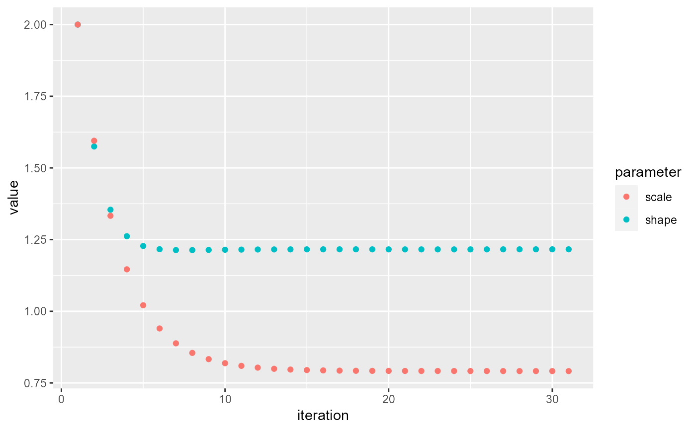 #> shape scale
#> 36 1.545727 0.6636448
# }
# Clustering the probabilities first
allClust <- clusterInfectors(nbResultsNoT, indIDVar = "individualID", pVar = "pScaled",
clustMethod = "hc_absolute", cutoff = 0.05)
performPEM(allClust[allClust$cluster == 1, ], indIDVar = "individualID",
timeDiffVar = "infectionDiffY", pVar = "pScaled",
initialPars = c(2, 2), shift = 0, plot = TRUE)
#> shape scale
#> 36 1.545727 0.6636448
# }
# Clustering the probabilities first
allClust <- clusterInfectors(nbResultsNoT, indIDVar = "individualID", pVar = "pScaled",
clustMethod = "hc_absolute", cutoff = 0.05)
performPEM(allClust[allClust$cluster == 1, ], indIDVar = "individualID",
timeDiffVar = "infectionDiffY", pVar = "pScaled",
initialPars = c(2, 2), shift = 0, plot = TRUE)
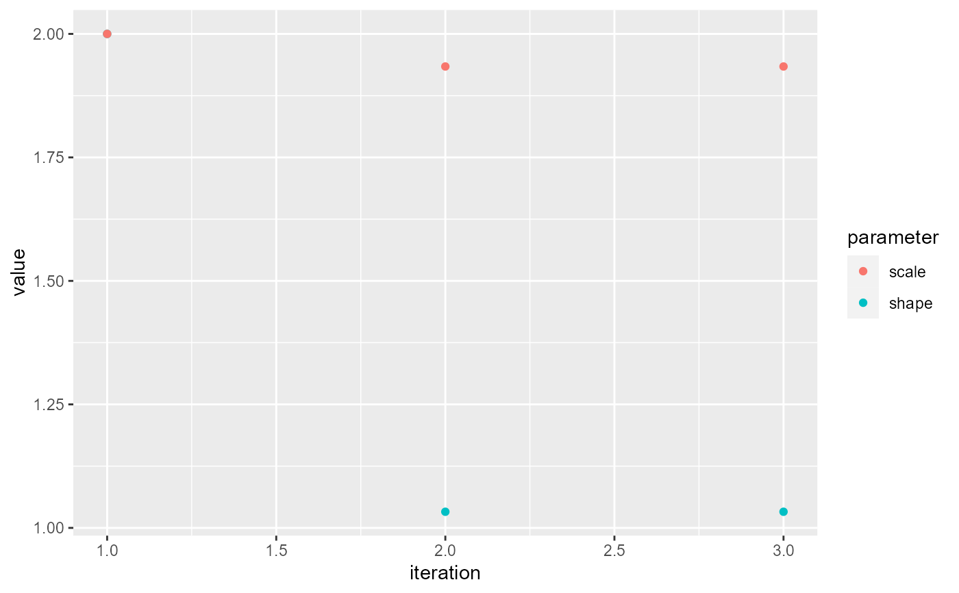 #> shape scale
#> 5 1.141596 1.778675
# \donttest{
# The above is equivalent to the following code using the function estimateSI()
# though the plot will not be printed and more details will be added
estimateSI(nbResultsNoT, indIDVar = "individualID", timeDiffVar = "infectionDiffY",
pVar = "pScaled", clustMethod = "hc_absolute", cutoff = 0.05,
initialPars = c(2, 2))
#>
|
| | 0%
|
|======================================================================| 100%
#> clustMethod cutoff nIndividuals nInfectors pCluster shape scale
#> 1 hc_absolute 0.05 77 1 0.7777778 1.141596 1.778675
#> meanSI medianSI sdSI
#> 1 2.030529 1.477798 1.900434
# }
#> shape scale
#> 5 1.141596 1.778675
# \donttest{
# The above is equivalent to the following code using the function estimateSI()
# though the plot will not be printed and more details will be added
estimateSI(nbResultsNoT, indIDVar = "individualID", timeDiffVar = "infectionDiffY",
pVar = "pScaled", clustMethod = "hc_absolute", cutoff = 0.05,
initialPars = c(2, 2))
#>
|
| | 0%
|
|======================================================================| 100%
#> clustMethod cutoff nIndividuals nInfectors pCluster shape scale
#> 1 hc_absolute 0.05 77 1 0.7777778 1.141596 1.778675
#> meanSI medianSI sdSI
#> 1 2.030529 1.477798 1.900434
# }